Filtering data is a crucial step in any data analysis process, and when working with time-based data in Excel, being able to filter values by a specific time range can be particularly useful. Whether you're tracking website traffic, sales data, or productivity metrics, Excel provides several ways to filter your data based on time ranges. In this article, we'll explore five methods to filter Excel values by a time range, from basic filtering techniques to more advanced formulas and pivot tables.
Method 1: Basic Filtering with AutoFilter

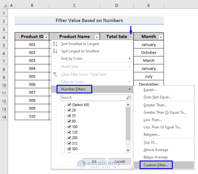
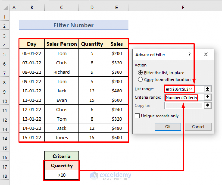
The simplest way to filter data by a time range in Excel is by using the AutoFilter feature. To use AutoFilter, select the header row of your data range, go to the "Data" tab in the ribbon, and click on the "Filter" button. This will enable filtering for your data range, and you'll see dropdown arrows appear in the header row.
Click on the dropdown arrow in the date column, and you'll see a menu with options to filter by specific dates or date ranges. You can select "Custom" to open the "Custom AutoFilter" dialog box, where you can specify a custom date range using the "is after or equal to" and "is before or equal to" options.
Step-by-Step Instructions:
Select the header row of your data range. Go to the "Data" tab in the ribbon. Click on the "Filter" button. Click on the dropdown arrow in the date column. Select "Custom" and specify your custom date range.
Method 2: Using Excel Formulas with INDEX and MATCH
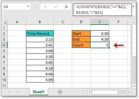
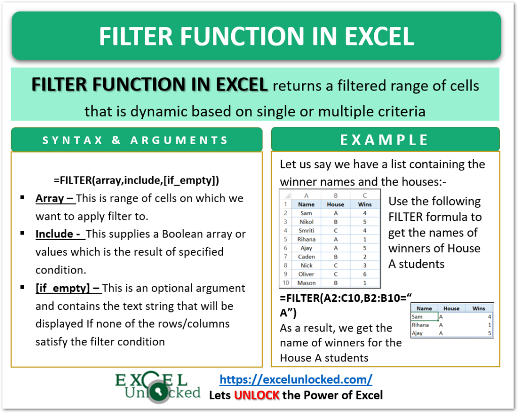
If you need more flexibility in filtering your data, you can use Excel formulas to create a dynamic filter. One approach is to use the INDEX and MATCH functions to extract data that falls within a specific time range.
Assuming your data is in columns A (date) and B (value), and you want to filter data between two dates (startdate and enddate), you can use the following formula:
=INDEX(B:B, MATCH(1, (A:A >= startdate) (A:A <= enddate), 0))
This formula uses the INDEX function to return the value in column B that corresponds to the row where the date in column A falls within the specified range.
Step-by-Step Instructions:
Enter the startdate and enddate in two separate cells. Enter the formula =INDEX(B:B, MATCH(1, (A:A >= startdate) (A:A <= enddate), 0)) in the cell where you want to display the filtered value. Press Enter to get the result.
Method 3: Using Excel PivotTables

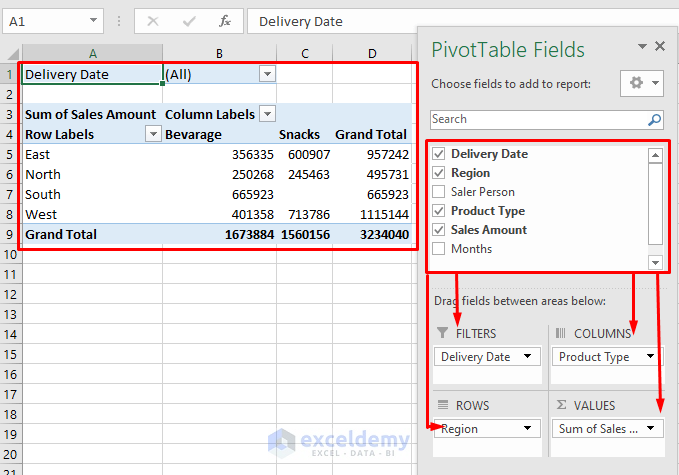
PivotTables are a powerful tool in Excel that allow you to summarize and analyze large datasets. You can use PivotTables to filter data by a time range by creating a date-based filter.
To create a PivotTable, select your data range, go to the "Insert" tab in the ribbon, and click on the "PivotTable" button. Then, drag the date field to the "Filters" area of the PivotTable and select the date range you want to filter by.
Step-by-Step Instructions:
Select your data range. Go to the "Insert" tab in the ribbon. Click on the "PivotTable" button. Drag the date field to the "Filters" area of the PivotTable. Select the date range you want to filter by.
Method 4: Using Excel Power Query
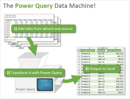
Excel Power Query is a powerful data manipulation tool that allows you to filter, transform, and load data from various sources. You can use Power Query to filter data by a time range by creating a query that extracts data between two dates.
To create a query, select your data range, go to the "Data" tab in the ribbon, and click on the "From Table/Range" button. Then, click on the "Filter" button and select the date range you want to filter by.
Step-by-Step Instructions:
Select your data range. Go to the "Data" tab in the ribbon. Click on the "From Table/Range" button. Click on the "Filter" button. Select the date range you want to filter by.
Method 5: Using Excel VBA Macros

If you need to automate the filtering process or create a custom filter, you can use Excel VBA macros. VBA macros allow you to write code that interacts with your Excel spreadsheet and performs tasks automatically.
To create a macro, open the Visual Basic Editor by pressing Alt + F11 or navigating to Developer > Visual Basic in the ribbon. Then, create a new module and write the code that filters your data by a time range.
Step-by-Step Instructions:
Open the Visual Basic Editor. Create a new module. Write the code that filters your data by a time range. Save the macro.
Conclusion
Filtering data by a time range is a common task in Excel, and there are several ways to achieve it. From basic filtering techniques to more advanced formulas and pivot tables, you can choose the method that best suits your needs. Whether you're working with small datasets or large datasets, these methods will help you extract the data you need and gain insights into your data. By mastering these techniques, you'll become more efficient in your data analysis tasks and make better decisions based on your data.
Gallery of 5 Ways To Filter Excel Values By Time Range

